00_Introduction_Computational_Graphs.ipynb

{
 "cells": [
  {
   "cell_type": "raw",
   "metadata": {},
   "source": [
    "---\n",
    "title: 01 Introduction to Computational Graphs\n",
    "description: A basic tutorial to learn about computational graphs\n",
    "---"
   ]
  },
  {
   "cell_type": "markdown",
   "metadata": {},
   "source": [
    "<a href=\"https://colab.research.google.com/drive/1eG1AF36Wa0EaANandAhrsbC3j04487SH?usp=sharing\" target=\"_blank\"><img align=\"left\" alt=\"Colab\" title=\"Open in Colab\" src=\"https://colab.research.google.com/assets/colab-badge.svg\"></a>"
   ]
  },
  {
   "cell_type": "markdown",
   "metadata": {
    "id": "_MbzfbWoqAaR"
   },
   "source": [
    "## Introduction to Computational Graphs with PyTorch\n",
    "\n",
    "by [Elvis Saravia](https://twitter.com/omarsar0)\n",
    "\n",
    "\n",
    "In this notebook we provide a short introduction and overview of computational graphs using PyTorch.\n",
    "\n",
    "There are several materials online that cover theory on the topic of computational graphs. However, I think it's much easier to learn the concept using code. I attempt to bridge the gap here which should be useful for beginner students.  \n",
    "\n",
    "Inspired by Olah's article [\"Calculus on Computational Graphs: Backpropagation\"](https://colah.github.io/posts/2015-08-Backprop/), I've put together a few code snippets to get you started with computationsl graphs with PyTorch. This notebook should complement that article, so refer to it for more comprehensive explanations. In fact, I've tried to simplify the explanations and refer to them here."
   ]
  },
  {
   "cell_type": "markdown",
   "metadata": {
    "id": "IGzBSo7H6xKu"
   },
   "source": [
    "### Why Computational Graphs?"
   ]
  },
  {
   "cell_type": "markdown",
   "metadata": {
    "id": "lkFMbiPDrGIp"
   },
   "source": [
    "When talking about neural networks in any context, [backpropagation](https://en.wikipedia.org/wiki/Backpropagation) is an important topic to understand because it is the algorithm used for training deep neural networks. \n",
    "\n",
    "Backpropagation is used to calculate derivatives which is what you need to keep optimizing parameters of the model and allowing the model to learn on the task at hand. \n",
    "\n",
    "Many of the deep learning frameworks today like PyTorch does the backpropagation out-of-the-box using [**automatic differentiation**](https://pytorch.org/tutorials/beginner/blitz/autograd_tutorial.html). \n",
    "\n",
    "To better understand how this is done it's important to talk about **computational graphs** which defines the flow of computations that are carried out throughout the network. Along the way we will use `torch.autograd` to demonstrate in code how this works.  "
   ]
  },
  {
   "cell_type": "markdown",
   "metadata": {
    "id": "YXjsI50-sMAa"
   },
   "source": [
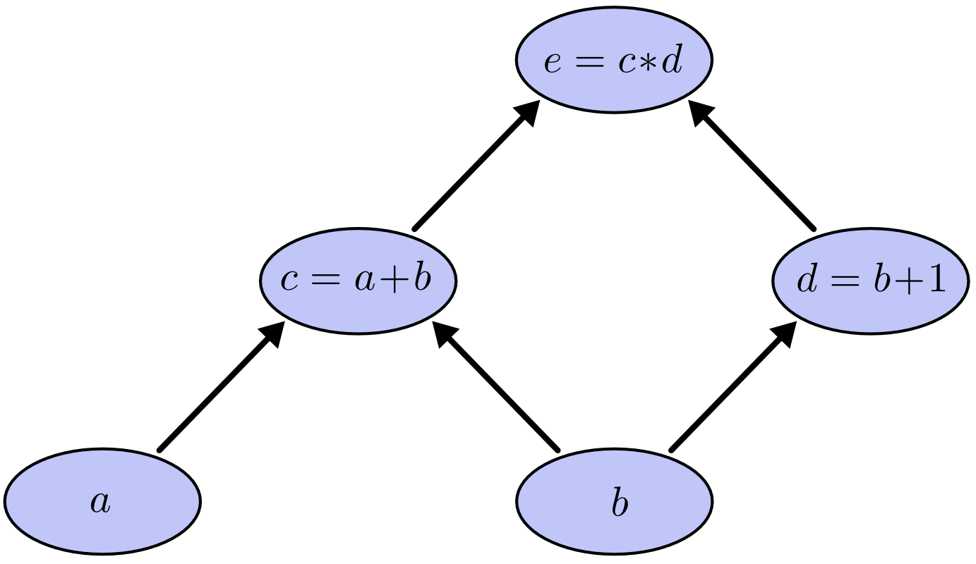
    "### Getting Started\n",
    "\n",
    "Inspired by Olah's article on computational graphs, let's look at the following expression $e = (a + b) * (b+1)$. It helps to break it down to the following operations:\n",
    "\n",
    "$$\n",
    "\\begin{aligned}&c=a+b \\\\&d=b+1 \\\\&e=c * d\\end{aligned}\n",
    "$$"
   ]
  },
  {
   "cell_type": "markdown",
   "metadata": {
    "id": "s0EG6DhnsnTm"
   },
   "source": [
    "This is not a neural network of any sort. We are just going through a very simple example of a chain of operations which you can be represented with computational graphs. \n",
    "\n",
    "Let's visualize these operations using a computational graph. Computational graphs contain **nodes** which can represent and input (tensor, matrix, vector, scalar) or **operation** that can be the input to another node. The nodes are connected by **edges**, which represent a function argument, they are pointers to nodes. Note that the computation graphs are directed and acyclic. The computational graph for our example looks as follows:\n",
    "\n",
    "![](https://colah.github.io/posts/2015-08-Backprop/img/tree-def.png)\n",
    "\n",
    "*Source: Christopher Olah (2015)*"
   ]
  },
  {
   "cell_type": "markdown",
   "metadata": {
    "id": "m9VvF4CVtW0s"
   },
   "source": [
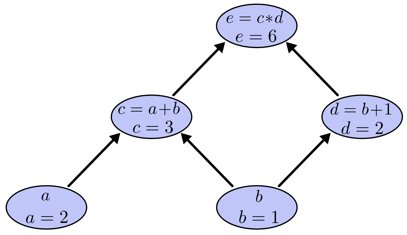
    "We can evaluate the expression by setting our input variables as follows: $a=2$ and $b=1$. This will allow us to compute nodes up through the graph as shown in the computational graph above.  \n",
    "\n",
    "Rather than doing this by hand, we can use the automatic differentation engine provided by PyTorch. \n",
    "\n",
    "Let's import PyTorch first:"
   ]
  },
  {
   "cell_type": "code",
   "execution_count": null,
   "metadata": {
    "id": "YuD6zdWZp7DP"
   },
   "outputs": [],
   "source": [
    "import torch"
   ]
  },
  {
   "cell_type": "markdown",
   "metadata": {
    "id": "b7EKlMrouClt"
   },
   "source": [
    "Define the inputs like this:"
   ]
  },
  {
   "cell_type": "code",
   "execution_count": null,
   "metadata": {
    "id": "OZ2pB2A3uEQZ"
   },
   "outputs": [],
   "source": [
    "a = torch.tensor([2.], requires_grad=True)\n",
    "b = torch.tensor([1.], requires_grad=True)"
   ]
  },
  {
   "cell_type": "markdown",
   "metadata": {
    "id": "Zm6Xl05quGZL"
   },
   "source": [
    "Note that we used `requires_grad=True` to tell the autograd engine that every operation on them should be tracked. \n",
    "\n",
    "These are the operations in code:"
   ]
  },
  {
   "cell_type": "code",
   "execution_count": null,
   "metadata": {
    "id": "XwXomBUxu1Ib"
   },
   "outputs": [],
   "source": [
    "c = a + b\n",
    "d = b + 1\n",
    "e = c * d\n",
    "\n",
    "# grads populated for non-leaf nodes\n",
    "c.retain_grad()\n",
    "d.retain_grad()\n",
    "e.retain_grad()"
   ]
  },
  {
   "cell_type": "markdown",
   "metadata": {
    "id": "UzCLJvMku46r"
   },
   "source": [
    "Note that we used `.retain_grad()` to allow gradients to be stored for non-leaf nodes as we are interested in inpecting those as well.\n",
    "\n",
    "Now that we have our computational graph, we can check the result when evaluating the expression:"
   ]
  },
  {
   "cell_type": "code",
   "execution_count": null,
   "metadata": {
    "colab": {
     "base_uri": "https://localhost:8080/"
    },
    "id": "4t-uhE6vvH2j",
    "outputId": "e834dbd0-0d8b-4123-d8fe-b9192aeaba9c"
   },
   "outputs": [
    {
     "name": "stdout",
     "output_type": "stream",
     "text": [
      "tensor([6.], grad_fn=<MulBackward0>)\n"
     ]
    }
   ],
   "source": [
    "print(e)"
   ]
  },
  {
   "cell_type": "markdown",
   "metadata": {
    "id": "5eWub17iwi2L"
   },
   "source": [
    "The output is a tensor with the value of `6.`, which verifies the results here: \n",
    "\n",
    "![](https://colah.github.io/posts/2015-08-Backprop/img/tree-eval.png)\n",
    "*Source: Christopher Olah (2015)*"
   ]
  },
  {
   "cell_type": "markdown",
   "metadata": {
    "id": "tjX3LCRmw22a"
   },
   "source": [
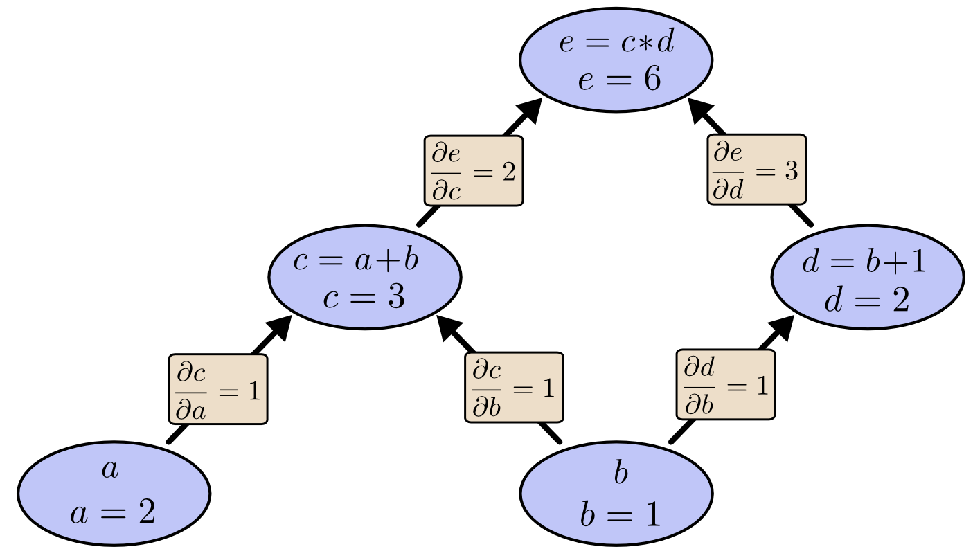
    "### Derivatives on Computational Graphs\n",
    "\n",
    "Using the concept of computational graphs we are now interested in evaluating the **partial derivatives** of the edges of the graph. This will help in gathering the gradients of the graph. Remember that gradients are what we use to train the neural network and those calculations can be taken care of by the automatic differentation engine. \n",
    "\n",
    "The intuition is: we want to know, for example, if $a$ directly affects $c$, how does it affect it. In other words, if we change $a$ a little, how does $c$ change. This is referred to as the partial derivative of $c$ with respect to $a$.\n",
    "\n",
    "You can work this by hand, but the easy way to do this with PyTorch is by calling `.backward()` on $e$ and let the engine figure out the values. The `.backward()` signals the autograd engine to calculate the gradients and store them in the respective tensors’ `.grad` attribute.\n",
    "\n",
    "Let's do that now:"
   ]
  },
  {
   "cell_type": "code",
   "execution_count": null,
   "metadata": {
    "id": "Nc6lnO5yy1Cq"
   },
   "outputs": [],
   "source": [
    "e.backward()"
   ]
  },
  {
   "cell_type": "markdown",
   "metadata": {
    "id": "hxbtx6OCy3I8"
   },
   "source": [
    "Now, let’s say we are interested in the derivative of $e$ with respect to $a$, how do we obtain this? In other words, we are looking for $\\frac{\\partial e}{\\partial a}$."
   ]
  },
  {
   "cell_type": "markdown",
   "metadata": {
    "id": "NvQcK9LTzD34"
   },
   "source": [
    "Using PyTorch, we can do this by calling `a.grad`:"
   ]
  },
  {
   "cell_type": "code",
   "execution_count": null,
   "metadata": {
    "colab": {
     "base_uri": "https://localhost:8080/"
    },
    "id": "5NWnWDg4zHDn",
    "outputId": "40cfe57c-23ee-4142-e62f-f7ef4b65fff0"
   },
   "outputs": [
    {
     "name": "stdout",
     "output_type": "stream",
     "text": [
      "tensor([2.])\n"
     ]
    }
   ],
   "source": [
    "print(a.grad)"
   ]
  },
  {
   "cell_type": "markdown",
   "metadata": {
    "id": "c05nEObzzbPn"
   },
   "source": [
    "It is important to understand the intuition behind this. Olah puts it best:\n",
    "\n",
    ">Let’s consider how $e$ is affected by $a$. If we change $a$ at a speed of 1, $c$ also changes at a speed of $1$. In turn, $c$ changing at a speed of $1$ causes $e$ to change at a speed of $2$. So $e$ changes at a rate of $1*2$ with respect to $a$.\n"
   ]
  },
  {
   "cell_type": "markdown",
   "metadata": {
    "id": "8xXLOU37BYOr"
   },
   "source": [
    "In other words, by hand this would be:\n",
    "\n",
    "$$\n",
    "\\frac{\\partial e}{\\partial \\boldsymbol{a}}=\\frac{\\partial e}{\\partial \\boldsymbol{c}} \\frac{\\partial \\boldsymbol{c}}{\\partial \\boldsymbol{a}} = 2 * 1\n",
    "$$"
   ]
  },
  {
   "cell_type": "markdown",
   "metadata": {
    "id": "A2iNJu6jzT5v"
   },
   "source": [
    "You can verify that this is correct by checking the manual calculations by Olah. Since $a$ is not directly connectected to $e$, we can use some special rule which allows to sum over all paths from one node to the other in the computational graph and mulitplying the derivatives on each edge of the path together.\n",
    "\n",
    "![](https://colah.github.io/posts/2015-08-Backprop/img/tree-eval-derivs.png)\n",
    "*Source: Christopher Olah (2015)*"
   ]
  },
  {
   "cell_type": "markdown",
   "metadata": {
    "id": "9uZE-Gl12cnB"
   },
   "source": [
    "To check that this holds, let look at another example. How about caluclating the derivative of $e$ with respect to $b$, i.e., $\\frac{\\partial e}{\\partial b}$?\n",
    "\n",
    "We can get that through `b.grad`:"
   ]
  },
  {
   "cell_type": "code",
   "execution_count": null,
   "metadata": {
    "colab": {
     "base_uri": "https://localhost:8080/"
    },
    "id": "2q11abV90d6i",
    "outputId": "11571cdc-7e55-43a9-931f-ec1ecf140efa"
   },
   "outputs": [
    {
     "name": "stdout",
     "output_type": "stream",
     "text": [
      "tensor([5.])\n"
     ]
    }
   ],
   "source": [
    "print(b.grad)"
   ]
  },
  {
   "cell_type": "markdown",
   "metadata": {
    "id": "2mGP1_iw0_ot"
   },
   "source": [
    "If you work it out by hand, you are basically doing the following:\n",
    "\n",
    "$$\n",
    "\\frac{\\partial e}{\\partial b}=1 * 2+1 * 3\n",
    "$$\n",
    "\n",
    "It indicates how $b$ affects $e$ through $c$ and $d$. We are essentially summing over paths in the computational graph."
   ]
  },
  {
   "cell_type": "markdown",
   "metadata": {
    "id": "sbJvhj5m13Zq"
   },
   "source": [
    "Here are all the gradients collected, including non-leaf nodes:"
   ]
  },
  {
   "cell_type": "code",
   "execution_count": null,
   "metadata": {
    "colab": {
     "base_uri": "https://localhost:8080/"
    },
    "id": "vrUxwsrd3-f-",
    "outputId": "cc63c914-b2e4-43b9-8c43-dcd70975e8b0"
   },
   "outputs": [
    {
     "name": "stdout",
     "output_type": "stream",
     "text": [
      "tensor([2.]) tensor([5.]) tensor([2.]) tensor([3.]) tensor([1.])\n"
     ]
    }
   ],
   "source": [
    "print(a.grad, b.grad, c.grad, d.grad, e.grad)"
   ]
  },
  {
   "cell_type": "markdown",
   "metadata": {
    "id": "HftIH5Mx4Pdj"
   },
   "source": [
    "You can use the computational graph above to verify that everything is correct. This is the power of computational graphs and how they are used by automatic differentation engines. It's also a very useful concept to understand when developing neural networks architectures and their correctness."
   ]
  },
  {
   "cell_type": "markdown",
   "metadata": {
    "id": "DxyJDoMOs1gu"
   },
   "source": [
    "### Next Steps\n",
    "\n",
    "In this notebook, I've provided a simple and intuitive explanation to the concept of computational graphs using PyTorch. I highly recommend to go through [Olah's article](https://colah.github.io/posts/2015-08-Backprop/) for more on the topic.\n",
    "\n",
    "In the next tutorial, I will be applying the concept of computational graphs to more advanced operations you typically see in a neural network. In fact, if you are interested in this, and you are feeling comfortable with the topic now, you can check out these two PyTorch tutorials:\n",
    "\n",
    "- [A gentle introduction to `torch.autograd`](https://pytorch.org/tutorials/beginner/blitz/autograd_tutorial.html)\n",
    "- [Automatic differentation with `torch.autograd`](https://pytorch.org/tutorials/beginner/basics/autogradqs_tutorial.html)\n",
    "\n",
    "And here are some other useful references used to put this article together:\n",
    "\n",
    "- [Hacker's guide to Neural Networks\n",
    "](http://karpathy.github.io/neuralnets/)\n",
    "- [Backpropagation calculus](https://www.youtube.com/watch?v=tIeHLnjs5U8&ab_channel=3Blue1Brown)\n",
    "\n"
   ]
  }
 ],
 "metadata": {
  "colab": {
   "name": "Introduction-Computational-Graphs.ipynb",
   "provenance": []
  },
  "kernelspec": {
   "display_name": "Python 3 (ipykernel)",
   "language": "python",
   "name": "python3"
  },
  "language_info": {
   "codemirror_mode": {
    "name": "ipython",
    "version": 3
   },
   "file_extension": ".py",
   "mimetype": "text/x-python",
   "name": "python",
   "nbconvert_exporter": "python",
   "pygments_lexer": "ipython3",
   "version": "3.9.12"
  }
 },
 "nbformat": 4,
 "nbformat_minor": 1
}