license: apache-2.0
datasets:
  - google/fleurs
metrics:
  - wer
  - accuracy
  - cer
pipeline_tag: automatic-speech-recognition
tags:
  - pitch
  - f0
  - echo
  - whiper
  - waveform
  - spectrogram
  - hilbert
  - asr
  - nlp
  - new
NLP/ASR multimodal modal with f0 modulated relative positional embeddings. For research/testing.
This plot illustrates the pattern similiarity of pitch and spectrogram. (librispeech - clean).
To explore the relationship between pitch and rotary embeddings, the model implements three complementary pitch based enhancements:
- Pitch modulated theta Pitch (f0) is used to modify the theta parameter, dynamically adjusting the rotary frequency.
- Direct similarity bias: A pitch based similarity bias is added directly to the attention mechanism.
- Variable radii in torch.polar: The unit circle radius (1.0) in the torch.polar calculation is replaced with variable radii derived from f0. This creates acoustically-weighted positional encodings, so each position in the embedding space reflects the acoustic prominence in the original speech. This approach effectively adds phase and amplitutde information without significant computational overhead.
The function torch.polar constructs a complex tensor from polar coordinates:
# torch.polar(magnitude, angle) returns:
result = magnitude * (torch.cos(angle) + 1j * torch.sin(angle))
So, for each element:
- magnitude is the modulus (radius, r)
- angle is the phase (theta, in radians)
- The result is:
r * exp(i * theta) = r * (cos(theta) + i * sin(theta))
Reference: PyTorch Documentation - torch.polar
Here are the abbreviated steps for replacing theta and radius in the rotary forward:
f0 = f0.to(device, dtype) # feature extracted during processing
f0_mean = f0.mean() # mean only used as theta in freqs calculation
theta = f0_mean + self.theta
## This can be just f0_mean or even perhaps f0 (per frame) and probably should for voice audio.
## In text, theta=10,000 sets the base frequency for positional encoding, ensuring a wide range of periodicities for long sequences. I'm not convinced by that arguement even for text.
## But.. for audio, especially speech, the relevant periodicities are determined by the pitch (f0), so using f0_mean (or even better, the local f0 per frame) might be more meaningful.

freqs = (theta / 220.0) * 700 * (torch.pow(10, torch.linspace(0, 2595 * torch.log10(torch.tensor(1 + 8000/700)), self.dim // 2) / 2595) - 1) / 1000
## This seems to give superior results compared to the standard freqs = 1. / (theta ** (torch.arange(0, dim, 2)[:(dim // 2)].float() / dim)).
## I thought a mel-scale version might be more perceptually meaningful for audio.. Hovering around 220.0 seems to be a sweet spot but I imagine this depends on dataset specifics. Whale speech might be different.

freqs = t[:, None] * freqs[None, :] # dont repeat or use some other method here

if self.radii and f0 is not None:
    radius = f0.to(device, dtype) # we want to avoid using the mean of f0 (or any stat or interpolation)
    if radius.shape[0] != x.shape[0]: # encoder outputs will already be the correct length
        F = radius.shape[0] / x.shape[0]
        idx = torch.arange(x.shape[0], device=f0.device)
        idx = (idx * F).long().clamp(0, radius.shape[0] - 1)
        radius = radius[idx]
    freqs = torch.polar(radius.unsqueeze(-1).expand_as(freqs), freqs)
else:
    freqs = torch.polar(torch.ones_like(freqs), freqs)
Approximation methods like using cos/sin projections or fixed rotation matrices typically assume a unit circle (radius=1.0) or only rotate, not scale. When we introduce a variable radius, those approximations break down and can't represent the scaling effect, only the rotation. When using a variable radius, we should use true complex multiplication to get correct results. Approximations that ignore the radius or scale after the rotation don't seem to capture the intended effect, leading to degraded or incorrect representations from my tests so far.
### Do not approximate:
#     radius = radius.unsqueeze(-1).expand_as(x_rotated[..., ::2])
#     x_rotated[..., ::2] = x_rotated[..., ::2] * radius
#     x_rotated[..., 1::2] = x_rotated[..., 1::2] * radius

###
    def apply_rotary(x, freqs):
        x1 = x[..., :freqs.shape[-1]*2]
        x2 = x[..., freqs.shape[-1]*2:]
        orig_shape = x1.shape
        if x1.ndim == 2:
            x1 = x1.unsqueeze(0)
        x1 = x1.float().reshape(*x1.shape[:-1], -1, 2).contiguous()
        x1 = torch.view_as_complex(x1) * freqs
        x1 = torch.view_as_real(x1).flatten(-2)
        x1 = x1.view(orig_shape)
        return torch.cat([x1.type_as(x), x2], dim=-1)
This approach respects both the rotation (phase) and the scaling (radius) for each token/head, so the rotary embedding is applied when the radius varies.
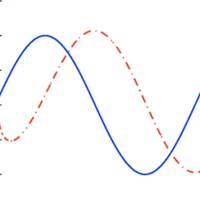
Each figure shows 4 subplots one for each of the first 4 dimensions of your embeddings in the test run. These visualizations show how pitch information modifies position encoding patterns in the model.
In each subplot:
- Thick solid lines: Standard RoPE rotations for even dimensions (no F0 adaptation)
- Thick dashed lines: Standard RoPE rotations for odd dimensions (no F0 adaptation)
- Thin solid lines: F0 RoPE rotations for even dimensions
- Thin dashed lines: F0 RoPE rotations for odd dimensions
Differences between thick and thin lines: This shows how much the F0 information is modifying the standard position encodings. Larger differences indicate stronger F0 adaptation.
Pattern changes: The standard RoPE (thick lines) show regular sinusoidal patterns, while the F0 RoPE (thin lines) show variations that correspond to the audio's pitch contour.
Dimension specific effects: Compared across four subplots to see if F0 affects different dimensions differently.
Position specific variations: In standard RoPE, frequency decreases with dimension index, but F0 adaptation modify this pattern.
The patterns below show how positions "see" each other in relation to theta and f0.
Bright diagonal line: Each position matches itself perfectly. Wider bright bands: Positions can "see" farther (good for long dependencies) but can be noisy. Narrow bands: More focus on nearby positions (good for local patterns)