Spaces:
Sleeping
Sleeping
File size: 6,142 Bytes
2999286 |
1 2 3 4 5 6 7 8 9 10 11 12 13 14 15 16 17 18 19 20 21 22 23 24 25 26 27 28 29 30 31 32 33 34 35 36 37 38 39 40 41 42 43 44 45 46 47 48 49 50 51 52 53 54 55 56 57 58 59 60 61 62 63 64 65 66 67 68 69 70 71 72 73 74 75 76 77 78 79 80 81 82 83 84 85 86 87 88 89 90 91 92 93 94 95 96 97 98 99 100 101 102 103 104 105 106 107 108 109 110 111 112 113 114 115 116 117 118 119 120 121 122 123 124 125 126 127 128 129 130 131 132 133 134 135 136 137 138 139 140 141 142 143 144 145 146 147 148 149 150 151 152 153 154 155 156 157 158 159 160 161 |
#!/usr/bin/env python
# coding: utf-8
# # Identifying Pseudo-Spatial Map
#
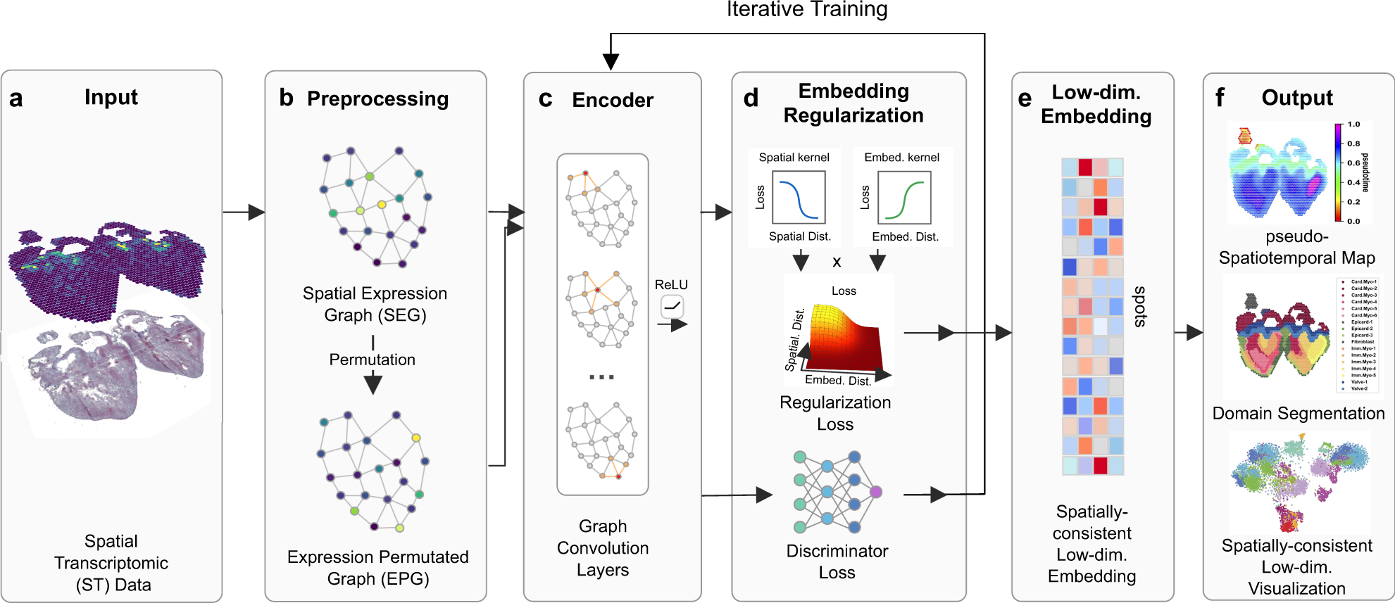
# SpaceFlow is Python package for identifying spatiotemporal patterns and spatial domains from Spatial Transcriptomic (ST) Data. Based on deep graph network, SpaceFlow provides the following functions:
# 1. Encodes the ST data into **low-dimensional embeddings** that reflecting both expression similarity and the spatial proximity of cells in ST data.
# 2. Incorporates **spatiotemporal** relationships of cells or spots in ST data through a **pseudo-Spatiotemporal Map (pSM)** derived from the embeddings.
# 3. Identifies **spatial domains** with spatially-coherent expression patterns.
#
# Check out [(Ren et al., Nature Communications, 2022)](https://www.nature.com/articles/s41467-022-31739-w) for the detailed methods and applications.
#
#
# 
#
# In[1]:
import omicverse as ov
#print(f"omicverse version: {ov.__version__}")
import scanpy as sc
#print(f"scanpy version: {sc.__version__}")
ov.utils.ov_plot_set()
# ## Preprocess data
#
# Here we present our re-analysis of 151676 sample of the dorsolateral prefrontal cortex (DLPFC) dataset. Maynard et al. has manually annotated DLPFC layers and white matter (WM) based on the morphological features and gene markers.
#
# This tutorial demonstrates how to identify spatial domains on 10x Visium data using STAGATE. The processed data are available at https://github.com/LieberInstitute/spatialLIBD. We downloaded the manual annotation from the spatialLIBD package and provided at https://drive.google.com/drive/folders/10lhz5VY7YfvHrtV40MwaqLmWz56U9eBP?usp=sharing.
# In[2]:
adata = sc.read_visium(path='data', count_file='151676_filtered_feature_bc_matrix.h5')
adata.var_names_make_unique()
# <div class="admonition warning">
# <p class="admonition-title">Note</p>
# <p>
# We introduced the spatial special svg calculation module prost in omicverse versions greater than `1.6.0` to replace scanpy's HVGs, if you want to use scanpy's HVGs you can set mode=`scanpy` in `ov.space.svg` or use the following code.
# </p>
# </div>
#
# ```python
# #adata=ov.pp.preprocess(adata,mode='shiftlog|pearson',n_HVGs=3000,target_sum=1e4)
# #adata.raw = adata
# #adata = adata[:, adata.var.highly_variable_features]
# ```
# In[3]:
sc.pp.calculate_qc_metrics(adata, inplace=True)
adata = adata[:,adata.var['total_counts']>100]
adata=ov.space.svg(adata,mode='prost',n_svgs=3000,target_sum=1e4,platform="visium",)
adata.raw = adata
adata = adata[:, adata.var.space_variable_features]
adata
# We read the ground truth area of our spatial data
# In[4]:
# read the annotation
import pandas as pd
import os
Ann_df = pd.read_csv(os.path.join('data', '151676_truth.txt'), sep='\t', header=None, index_col=0)
Ann_df.columns = ['Ground Truth']
adata.obs['Ground Truth'] = Ann_df.loc[adata.obs_names, 'Ground Truth']
sc.pl.spatial(adata, img_key="hires", color=["Ground Truth"])
# ## Training the SpaceFlow Model
#
# Here, we used `ov.space.pySpaceFlow` to construct a SpaceFlow Object and train the model.
#
# We need to store the space location info in `adata.obsm['spatial']`
# In[5]:
sf_obj=ov.space.pySpaceFlow(adata)
# We then train a spatially regularized deep graph network model to learn a low-dimensional embedding that reflecting both expression similarity and the spatial proximity of cells in ST data.
#
# Parameters:
# - `spatial_regularization_strength`: the strength of spatial regularization, the larger the more of the spatial coherence in the identified spatial domains and spatiotemporal patterns. (default: 0.1)
# - `z_dim`: the target size of the learned embedding. (default: 50)
# - `lr`: learning rate for optimizing the model. (default: 1e-3)
# - `epochs`: the max number of the epochs for model training. (default: 1000)
# - `max_patience`: the max number of the epoch for waiting the loss decreasing. If loss does not decrease for epochs larger than this threshold, the learning will stop, and the model with the parameters that shows the minimal loss are kept as the best model. (default: 50)
# - `min_stop`: the earliest epoch the learning can stop if no decrease in loss for epochs larger than the `max_patience`. (default: 100)
# - `random_seed`: the random seed set to the random generators of the `random`, `numpy`, `torch` packages. (default: 42)
# - `gpu`: the index of the Nvidia GPU, if no GPU, the model will be trained via CPU, which is slower than the GPU training time. (default: 0)
# - `regularization_acceleration`: whether or not accelerate the calculation of regularization loss using edge subsetting strategy (default: True)
# - `edge_subset_sz`: the edge subset size for regularization acceleration (default: 1000000)
#
# In[6]:
sf_obj.train(spatial_regularization_strength=0.1,
z_dim=50, lr=1e-3, epochs=1000,
max_patience=50, min_stop=100,
random_seed=42, gpu=0,
regularization_acceleration=True, edge_subset_sz=1000000)
# ## Calculated the Pseudo-Spatial Map
#
# Unlike the original SpaceFlow, we only need to use the `cal_PSM` function when calling SpaceFlow in omicverse to compute the pSM.
# In[7]:
sf_obj.cal_pSM(n_neighbors=20,resolution=1,
max_cell_for_subsampling=5000,psm_key='pSM_spaceflow')
# In[8]:
sc.pl.spatial(adata, color=['pSM_spaceflow','Ground Truth'],cmap='RdBu_r')
# ## Clustering the space
#
# We can use `GMM`, `leiden` or `louvain` to cluster the space.
#
# ```python
# sc.pp.neighbors(adata, n_neighbors=15, n_pcs=50,
# use_rep='spaceflow')
# ov.utils.cluster(adata,use_rep='spaceflow',method='louvain',resolution=1)
# ov.utils.cluster(adata,use_rep='spaceflow',method='leiden',resolution=1)
# ```
# In[9]:
ov.utils.cluster(adata,use_rep='spaceflow',method='GMM',n_components=7,covariance_type='full',
tol=1e-9, max_iter=1000, random_state=3607)
# In[10]:
sc.pl.spatial(adata, color=['gmm_cluster',"Ground Truth"])
# In[ ]:
|