|
--- |
|
license: apache-2.0 |
|
metrics: |
|
- accuracy |
|
- f1 |
|
- precision |
|
- recall |
|
library_name: transformers |
|
pipeline_tag: image-classification |
|
tags: |
|
- biology |
|
--- |
|
|
|
# Resumen |
|
|
|
El modelo fue entrenado usando el modelo base de VisionTransformer junto con el optimizador SAM de Google y la función de perdida Negative log likelihood, sobre los datos [Wildfire](https://drive.google.com/file/d/1TlF8DIBLAccd0AredDUimQQ54sl_DwCE/view?usp=sharing). Los resultados muestran que el clasificador alcanzó una precisión del 97% con solo 10 épocas de entrenamiento. |
|
La teoría de se muestra a continuación. |
|
 |
|
|
|
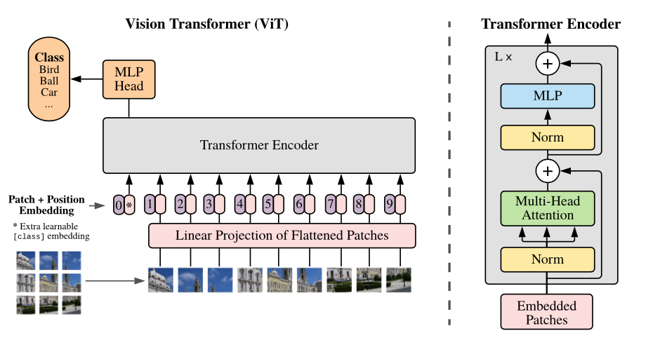
# VisionTransformer |
|
|
|
**Attention-based neural networks such as the Vision Transformer** (ViT) have recently attained state-of-the-art results on many computer vision benchmarks. Scale is a primary ingredient in attaining excellent results, therefore, understanding a model's scaling properties is a key to designing future generations effectively. While the laws for scaling Transformer language models have been studied, it is unknown how Vision Transformers scale. To address this, we scale ViT models and data, both up and down, and characterize the relationships between error rate, data, and compute. Along the way, we refine the architecture and training of ViT, reducing memory consumption and increasing accuracy of the resulting models. As a result, we successfully train a ViT model with two billion parameters, which attains a new state-of-the-art on ImageNet of 90.45% top-1 accuracy. The model also performs well for few-shot transfer, for example, reaching 84.86% top-1 accuracy on ImageNet with only 10 examples per class. |
|
|
|
|
|
|
|
[1] A. Dosovitskiy et al., “An Image is Worth 16x16 Words: Transformers for Image Recognition at Scale”. arXiv, el 3 de junio de 2021. Consultado: el 12 de noviembre de 2023. [En línea]. Disponible en: http://arxiv.org/abs/2010.11929 |
|
|
|
# Sharpness Aware Minimization (SAM) |
|
|
|
SAM simultaneously minimizes loss value and loss sharpness. In particular, it seeks parameters that lie in neighborhoods having uniformly low loss. SAM improves model generalization and yields SoTA performance for several datasets. Additionally, it provides robustness to label noise on par with that provided by SoTA procedures that specifically target learning with noisy labels. |
|
|
|
 |
|
|
|
*ResNet loss landscape at the end of training with and without SAM. Sharpness-aware updates lead to a significantly wider minimum, which then leads to better generalization properties.* |
|
|
|
[2] P. Foret, A. Kleiner, y H. Mobahi, “Sharpness-Aware Minimization For Efficiently Improving Generalization”, 2021. |
|
|
|
# The negative log likelihood loss |
|
|
|
It is useful to train a classification problem with $C$ classes. |
|
|
|
If provided, the optional argument weight should be a 1D Tensor assigning weight to each of the classes. This is particularly useful when you have an unbalanced training set. |
|
|
|
The input given through a forward call is expected to contain log-probabilities of each class. input has to be a Tensor of size either (minibatch, $C$ ) or ( minibatch, $C, d_1, d_2, \ldots, d_K$ ) with $K \geq 1$ for the $K$-dimensional case. The latter is useful for higher dimension inputs, such as computing NLL loss per-pixel for 2D images. |
|
|
|
Obtaining log-probabilities in a neural network is easily achieved by adding a LogSoftmax layer in the last layer of your network. You may use CrossEntropyLoss instead, if you prefer not to add an extra layer. |
|
|
|
The target that this loss expects should be a class index in the range $\[0, C-1\]$ where $C$ number of classes; if ignore_index is specified, this loss also accepts this class index (this index may not necessarily be in the class range). |
|
|
|
The unreduced (i.e. with reduction set to 'none ') loss can be described as: |
|
$$ |
|
\ell(x, y)=L=\left\{l_1, \ldots, l_N\right\}^{\top}, \quad l_n=-w_{y_n} x_{n, y_n}, \quad w_c=\text { weight }[c] \cdot 1 |
|
$$ |
|
where $x$ is the input, $y$ is the target, $w$ is the weight, and $N$ is the batch size. If reduction is not 'none' (default 'mean'), then |
|
$$ |
|
\ell(x, y)= \begin{cases}\sum_{n=1}^N \frac{1}{\sum_{n=1}^N w_{y_n}} l_n, & \text { if reduction }=\text { 'mean' } \\ \sum_{n=1}^N l_n, & \text { if reduction }=\text { 'sum' }\end{cases} |
|
$$ |
|
|
|
# Resultados obtenidos |
|
<img src="https://cdn-uploads.huggingface.co/production/uploads/64ff2131f7f3fa2d7fe256fc/CO6vFEjt3FkxB8JgZTbEd.png" width="500" /> |