Toy Examples with Code

Preamble

import numpy as np
from pysr import *

1. Simple search

Here's a simple example where we find the expression 2 cos(x3) + x0^2 - 2.

X = 2 * np.random.randn(100, 5)
y = 2 * np.cos(X[:, 3]) + X[:, 0] ** 2 - 2
model = PySRRegressor(binary_operators=["+", "-", "*", "/"])
model.fit(X, y)
print(model)

2. Custom operator

Here, we define a custom operator and use it to find an expression:

X = 2 * np.random.randn(100, 5)
y = 1 / X[:, 0]
model = PySRRegressor(
    binary_operators=["plus", "mult"],
    unary_operators=["inv(x) = 1/x"],
)
model.fit(X, y)
print(model)

3. Multiple outputs

Here, we do the same thing, but with multiple expressions at once, each requiring a different feature.

X = 2 * np.random.randn(100, 5)
y = 1 / X[:, [0, 1, 2]]
model = PySRRegressor(
    binary_operators=["plus", "mult"],
    unary_operators=["inv(x) = 1/x"],
)
model.fit(X, y)

4. Plotting an expression

Here, let's use the same equations, but get a format we can actually use and test. We can add this option after a search via the set_params function:

model.set_params(extra_sympy_mappings={"inv": lambda x: 1/x})
model.sympy()

If you look at the lists of expressions before and after, you will see that the sympy format now has replaced inv with 1/. We can again look at the equation chosen:

print(model)

For now, let's consider the expressions for output 0. We can see the LaTeX version of this with:

model.latex()[0]

or output 1 with model.latex()[1].

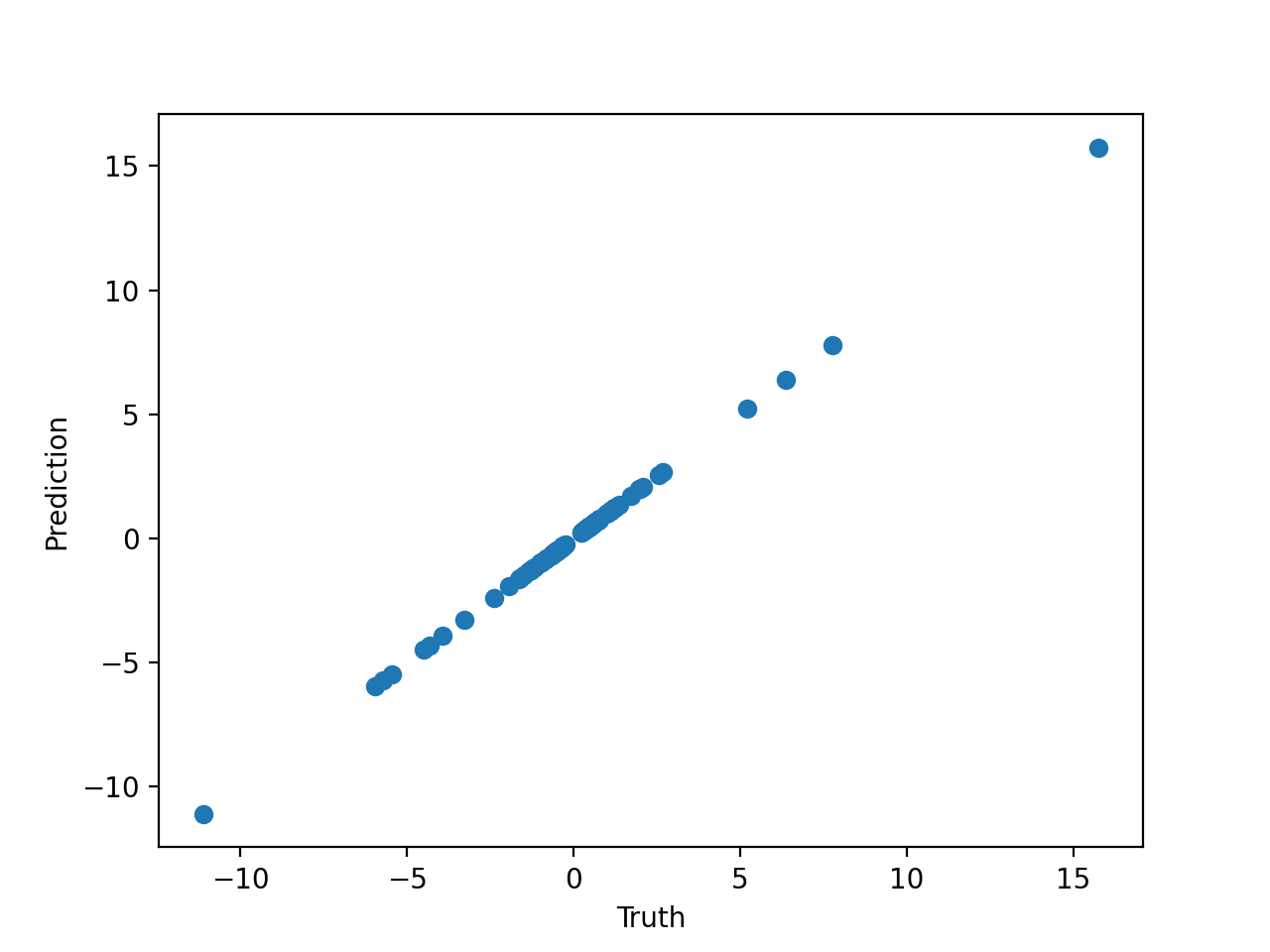
Let's plot the prediction against the truth:

from matplotlib import pyplot as plt
plt.scatter(y[:, 0], model(X)[:, 0])
plt.xlabel('Truth')
plt.ylabel('Prediction')
plt.show()

Which gives us:

5. Feature selection

PySR and evolution-based symbolic regression in general performs very poorly when the number of features is large. Even, say, 10 features might be too much for a typical equation search.

If you are dealing with high-dimensional data with a particular type of structure, you might consider using deep learning to break the problem into smaller "chunks" which can then be solved by PySR, as explained in the paper 2006.11287.

For tabular datasets, this is a bit trickier. Luckily, PySR has a built-in feature selection mechanism. Simply declare the parameter select_k_features=5, for selecting the most important 5 features.

Here is an example. Let's say we have 30 input features and 300 data points, but only 2 of those features are actually used:

X = np.random.randn(300, 30)
y = X[:, 3]**2 - X[:, 19]**2 + 1.5

Let's create a model with the feature selection argument set up:

model = PySRRegressor(
    binary_operators=["+", "-", "*", "/"],
    unary_operators=["exp"],
    select_k_features=5,
)

Now let's fit this:

model.fit(X, y)

Before the Julia backend is launched, you can see the string:

Using features ['x3', 'x5', 'x7', 'x19', 'x21']

which indicates that the feature selection (powered by a gradient-boosting tree) has successfully selected the relevant two features.

This fit should find the solution quickly, whereas with the huge number of features, it would have struggled.

This simple preprocessing step is enough to simplify our tabular dataset, but again, for more structured datasets, you should try the deep learning approach mentioned above.

6. Denoising

Many datasets, especially in the observational sciences, contain intrinsic noise. PySR is noise robust itself, as it is simply optimizing a loss function, but there are still some additional steps you can take to reduce the effect of noise.

One thing you could do, which we won't detail here, is to create a custom log-likelihood given some assumed noise model. By passing weights to the fit function, and defining a custom loss function such as loss="myloss(x, y, w) = w * (x - y)^2", you can define any sort of log-likelihood you wish. (However, note that it must be bounded at zero)

However, the simplest thing to do is preprocessing, just like for feature selection. To do this, set the parameter denoise=True. This will fit a Gaussian process (containing a white noise kernel) to the input dataset, and predict new targets (which are assumed to be denoised) from that Gaussian process.

For example:

X = np.random.randn(100, 5)
noise = np.random.randn(100) * 0.1
y = np.exp(X[:, 0]) + X[:, 1] + X[:, 2] + noise

Let's create and fit a model with the denoising argument set up:

model = PySRRegressor(
    binary_operators=["+", "-", "*", "/"],
    unary_operators=["exp"],
    denoise=True,
)
model.fit(X, y)
print(model)

If all goes well, you should find that it predicts the correct input equation, without the noise term!

7. Additional features

For the many other features available in PySR, please read the Options section.